L-Functions as Infinite Corrections

A Computational Tutorial

The Intuition Behind the Langlands Conjectures

My main motivation for this tutorial is to provide an introduction to the line of reasoning behind the (arithmetic) Langlands conjectures that I have not seen elsewhere, specifically the relationship between automorphic and motivic L-functions.

What are L-functions? Both zeta- and L-functions are functions in analytic number theory constructed to introduce correction terms to approximate constructions of mathematical data or objects (with the Riemann zeta function being the original use case). In the case of the Langlands conjectures, the crux of the intuition is that automorphic and motivic L-functions each provide correction terms in non-abelian harmonic analysis and algebraic geometry, respectively, due to very strong indicators that these correction terms amount to the same thing in number theory.

Why Use Correction Terms?

Suppose one has an approximation for some mathematical phenomenon that requires infinitely many correction terms to be exact. At first, one might think this approximation to be rather poor. However, many mathematical data, such as prime numbers, are infinite, so if one’s approximation and corrections are given by well-behaved and well-understood functions, they have the potential to provide concise descriptions of such data.

In analytic number theory, zeta-functions and L-functions are developed to introduce various kinds of correction terms.

The Riemann Zeta Function

Approximating the Distribution of Primes

The original zeta-function is the Riemann zeta function, ζ(z)

\(\zeta(s) = \sum_{n=1}^\infty n^{-s}\)

whose nontrivial zeros provide correction terms to approximations of the distribution of prime numbers.

As we know, the primes are of crucial importance, as they are the building blocks of all the composite natural numbers. However, what can we say, concretely, about all primes? Can we actually describe them, together, as a collection of mathematical data? Currently, we can only describe them conjecturally.

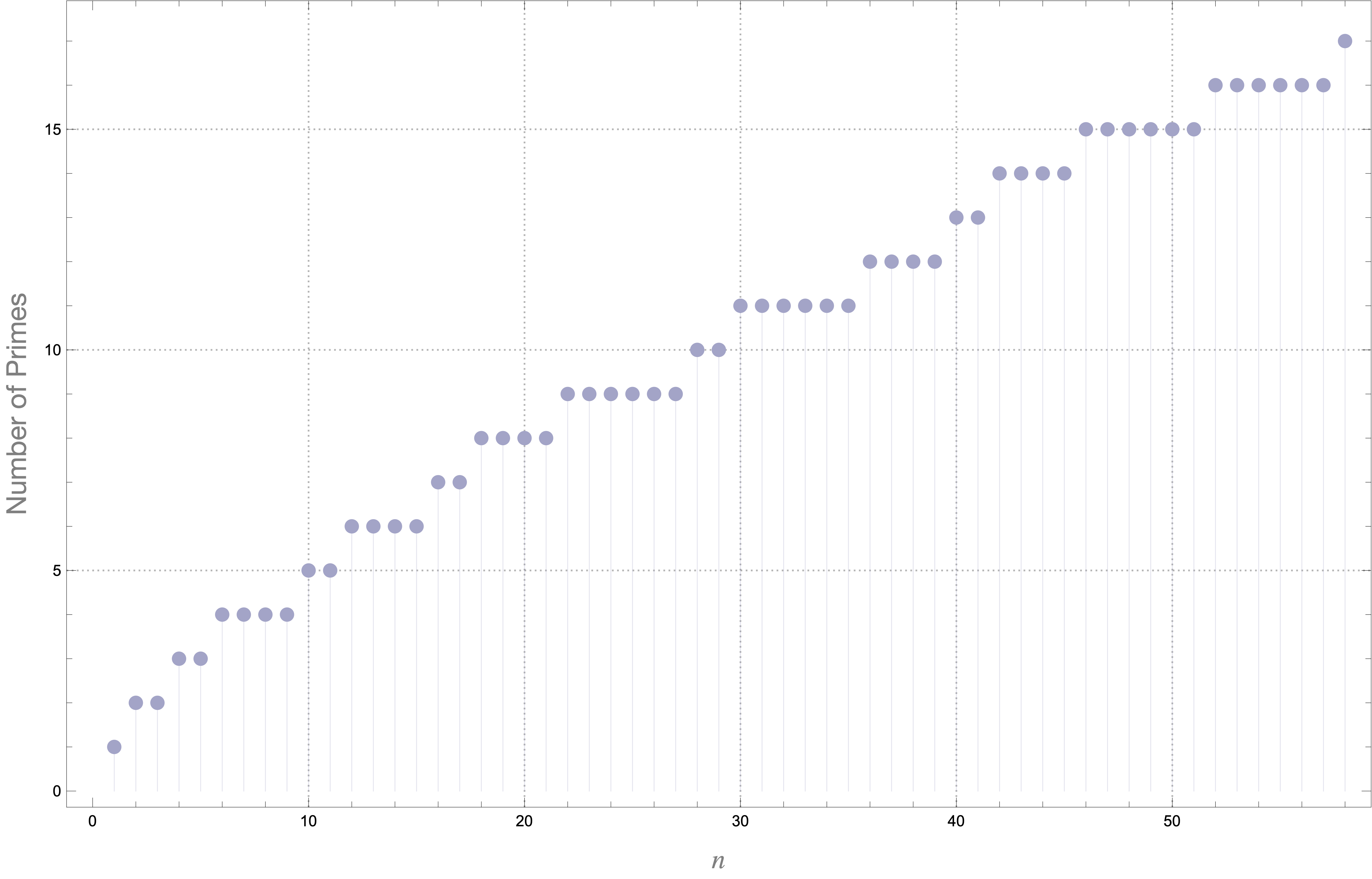
Suppose we were to ask how many primes appear after n natural numbers. We’ll call this our prime-counting function, π₀(x):

\(\pi_0(x)=|\{\mathrm{IsPrime}(n) \; | \; 1 \leq n \leq x\}|\)

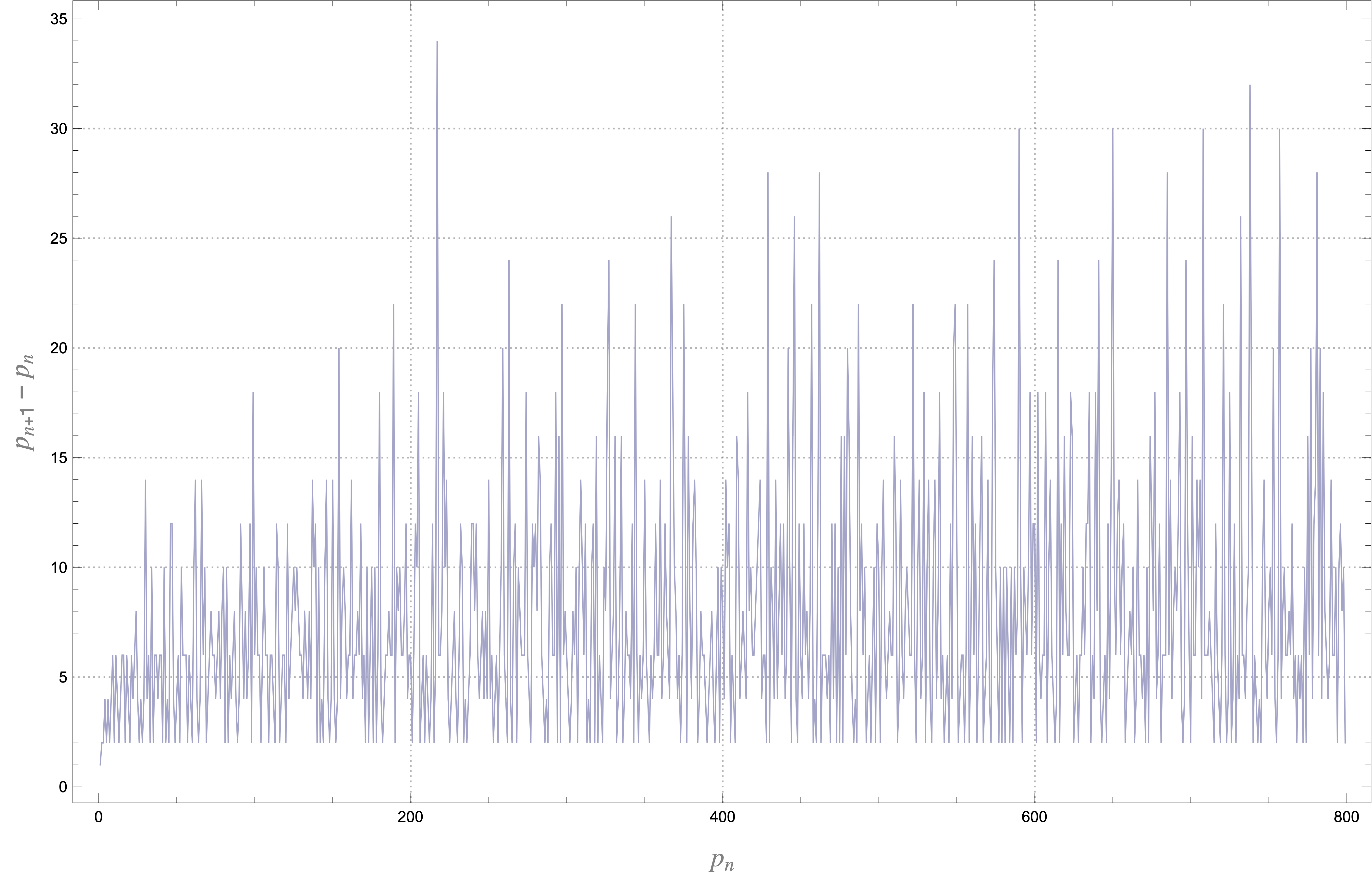
As one finds, the appearance of primes is somewhat difficult to predict. One doesn’t really know when the next prime will appear.

For instance, if one plots the distance between consecutive primes, one doesn’t find any immediately noticeable trend:

Let’s consider a rough approximation to π₀(x):

\(\mathrm{R}(x) = \sum_{n=1}^\infty \frac{\mu(n)}{n} \mathrm{li}(\sqrt[n]{x})\)

(where is the Möbius function and li is the logarithmic integral). As we can see, the approximation is very rough:

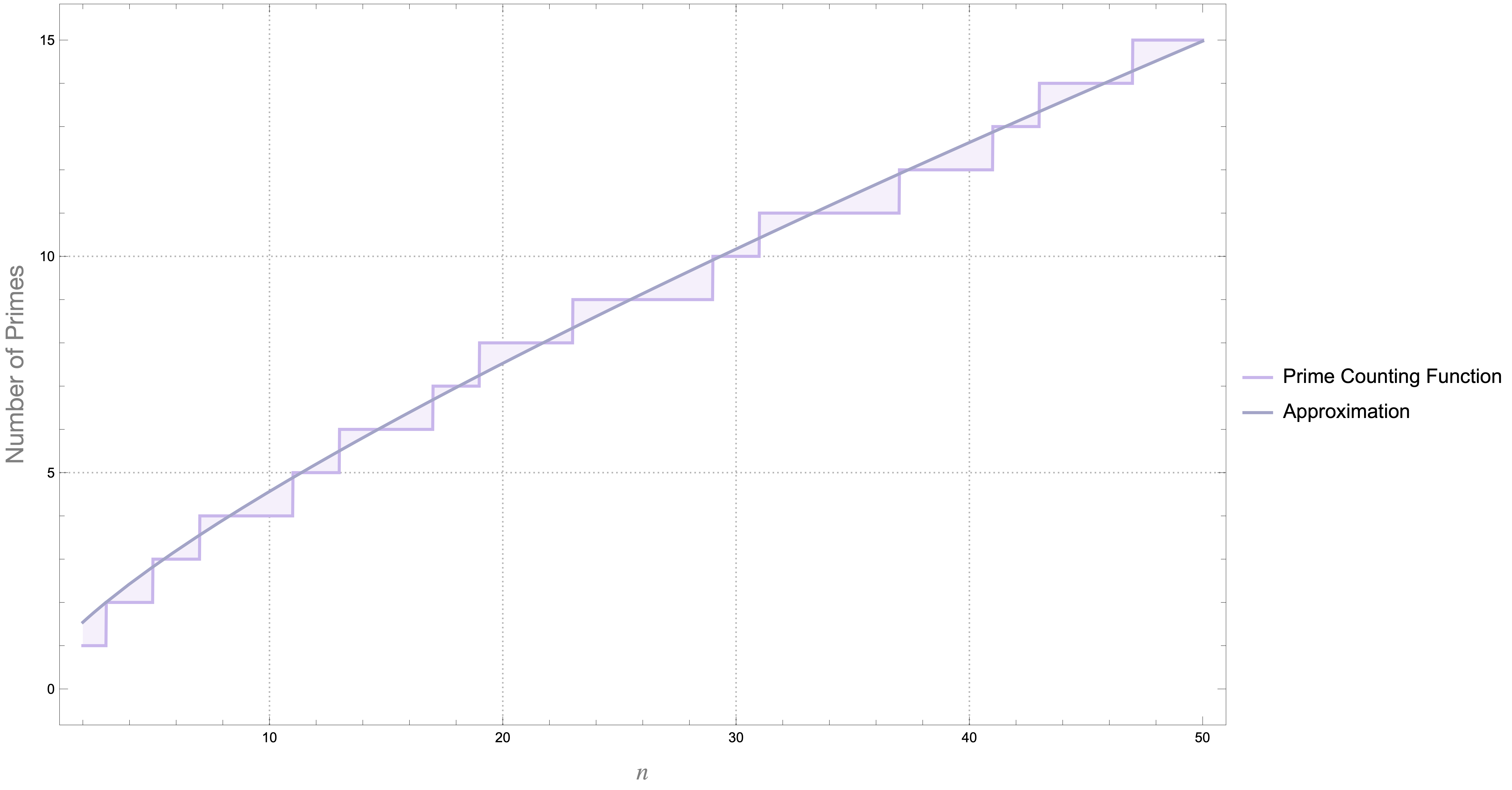
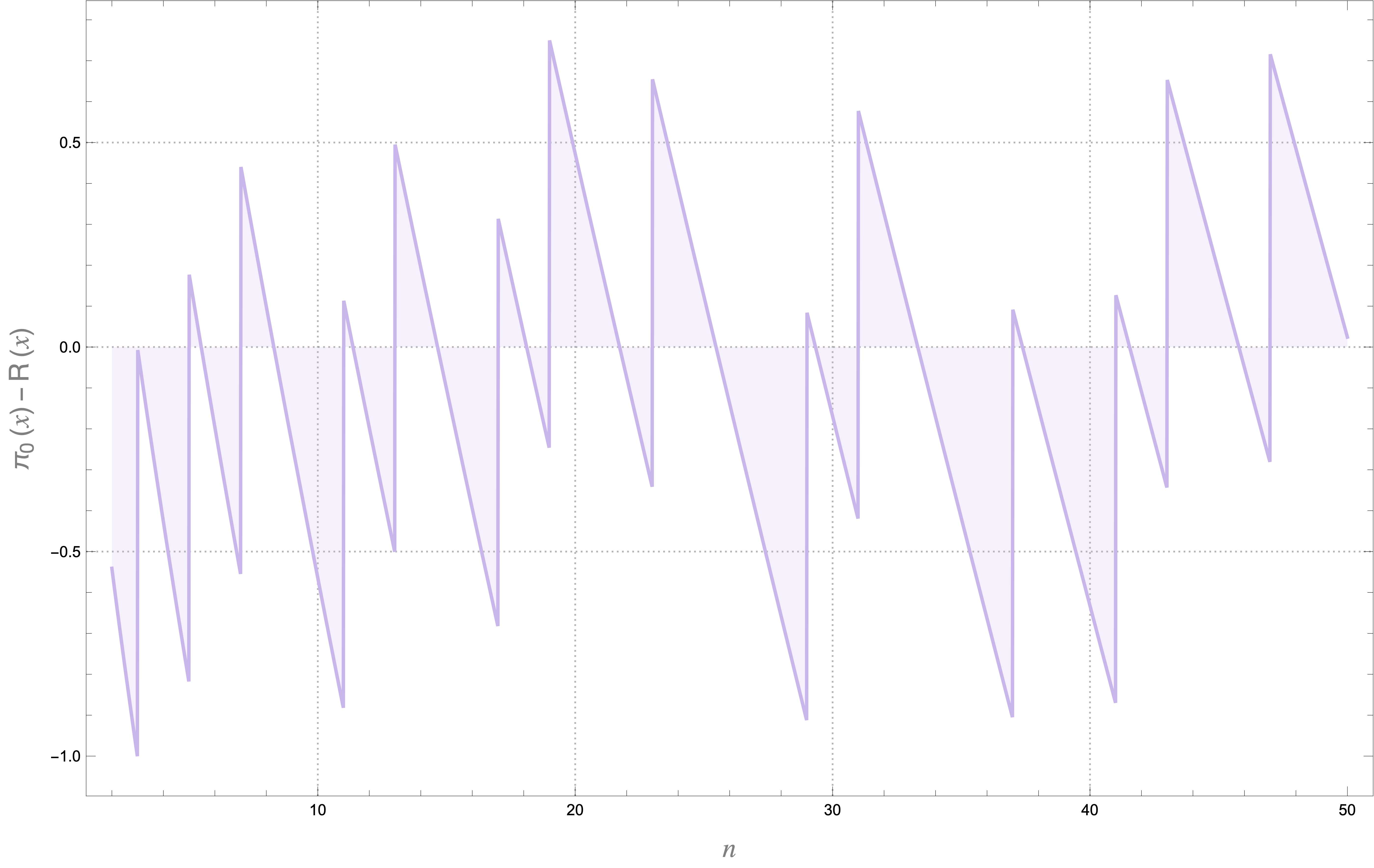
as there are rather grievous error terms:

Riemann Zeros and Correction Terms

However, it is believed that correction terms can be introduced to asymptotically make this approximation exact.

\(\pi_0(x) = \mathrm{R}(x) - \sum_{I(\rho)} \mathrm{Li}(x^\rho) - \mathrm{Li}(x^{1-\rho}) \)

Here the ρ terms are the non-trivial zeros of the Riemann zeta function! Empirically, we can see that introducing Riemann zeros into our approximation gradually improves it:

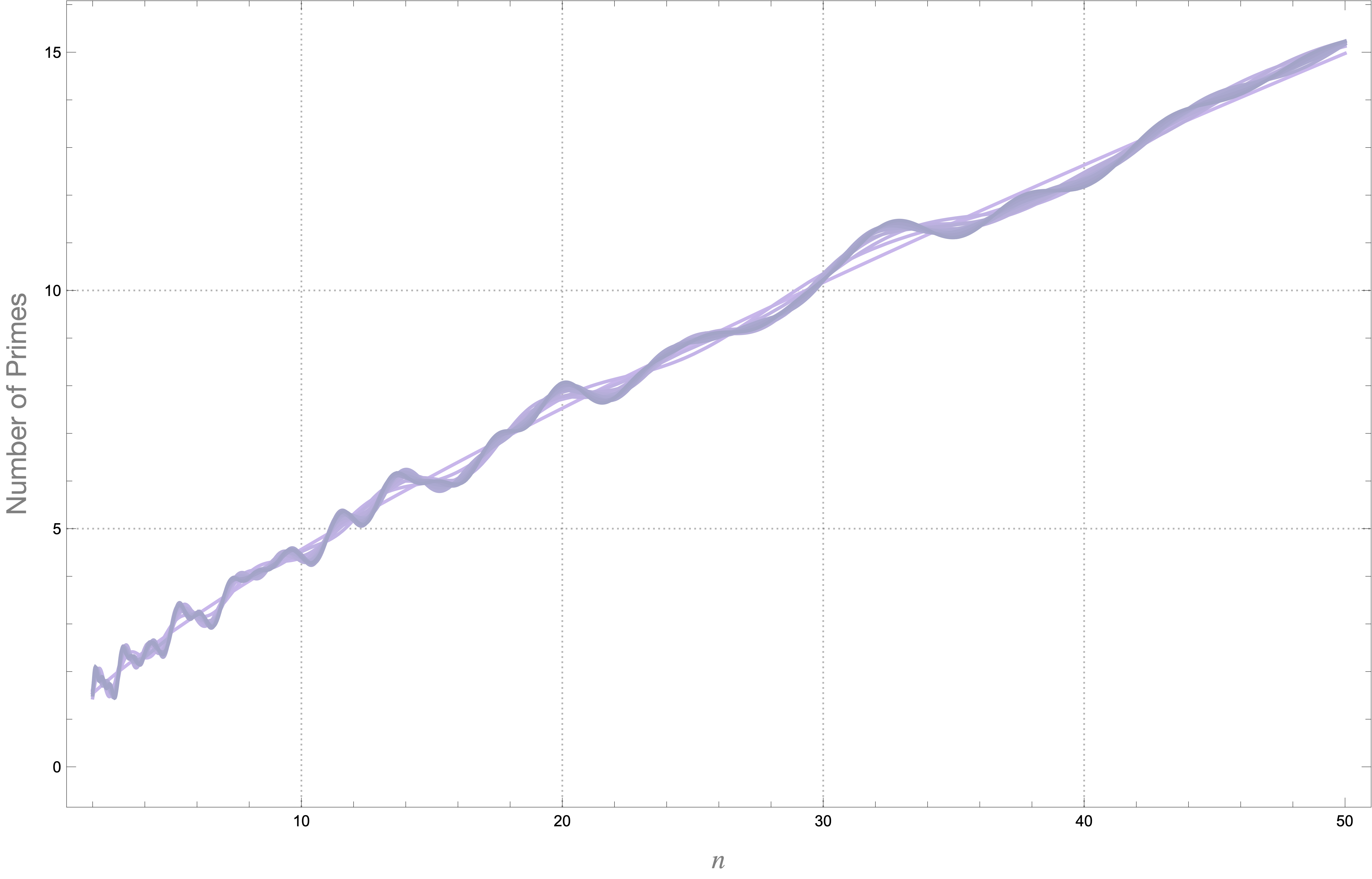
For comparison, here’s a plot of π₀(x) and R(x) with correction terms from the first 50 non-trivial Riemann zeros. The approximation is improving.

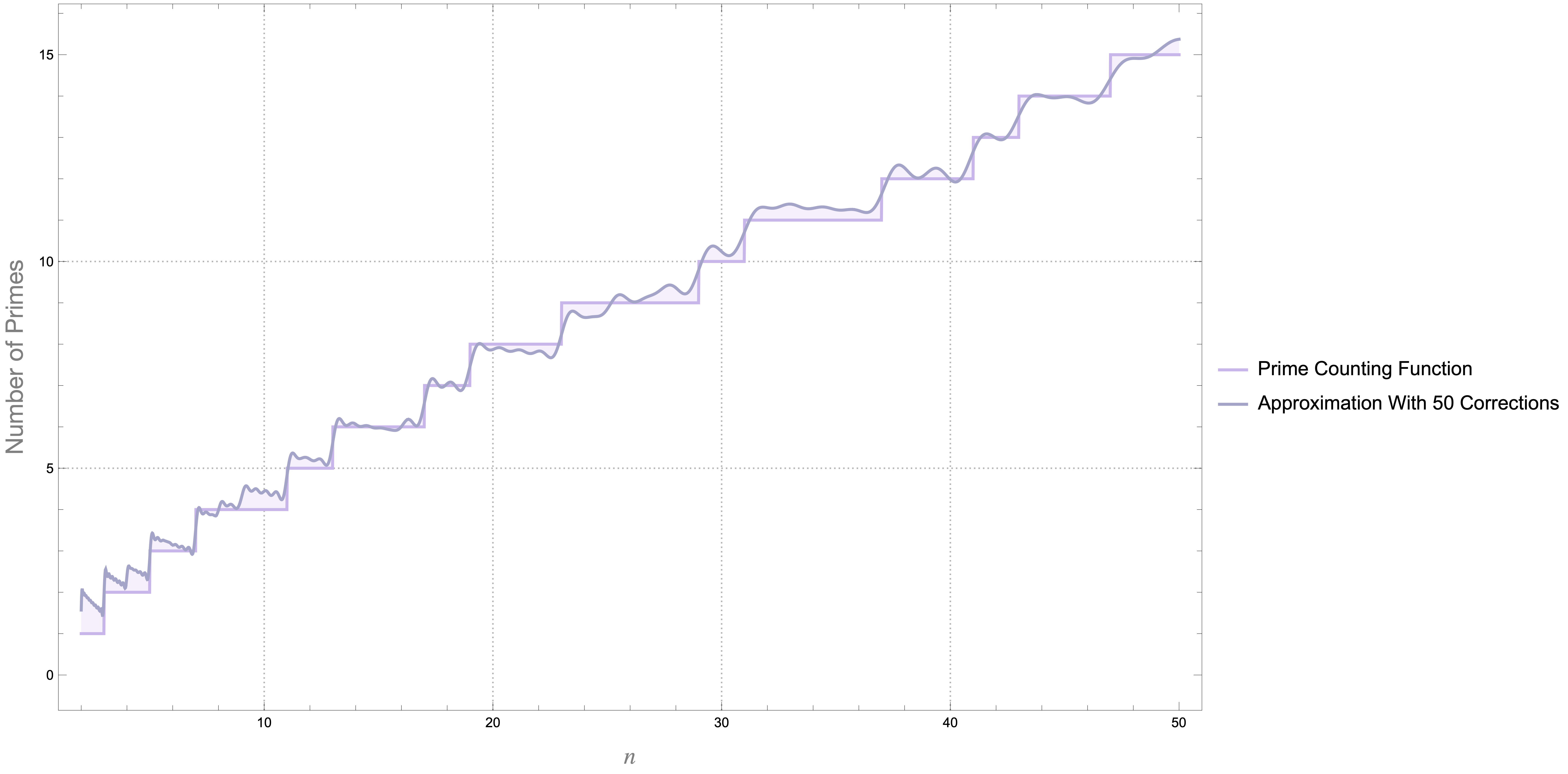
How many corrections are needed? Well, infinitely many. That’s why a zeta-function, with nice analytic properties, is important.

Next, we’ll consider two similar kinds of functions: motivic and automorphic L-functions.

Motivic L-Functions

Counting Solutions Mod p for Elliptic Curves

Suppose we have an elliptic curve and seek to count its solutions mod p or mod pⁿ. One key motivation for computing mod p is that it provides a tractable alternative to computing over fields such as the rationals, ℚ. Counting points on algebraic varieties over ℚ is a part of Diophantine geometry. Even for elliptic curves, it can be difficult, as each curve is given by a single equation with two unknowns. So, one reason why counting solutions mod p or mod pⁿ is easier is that the underlying field is more wieldy; it amounts to counting points over a finite field

\(\mathbb {F} _ {p^n}\)

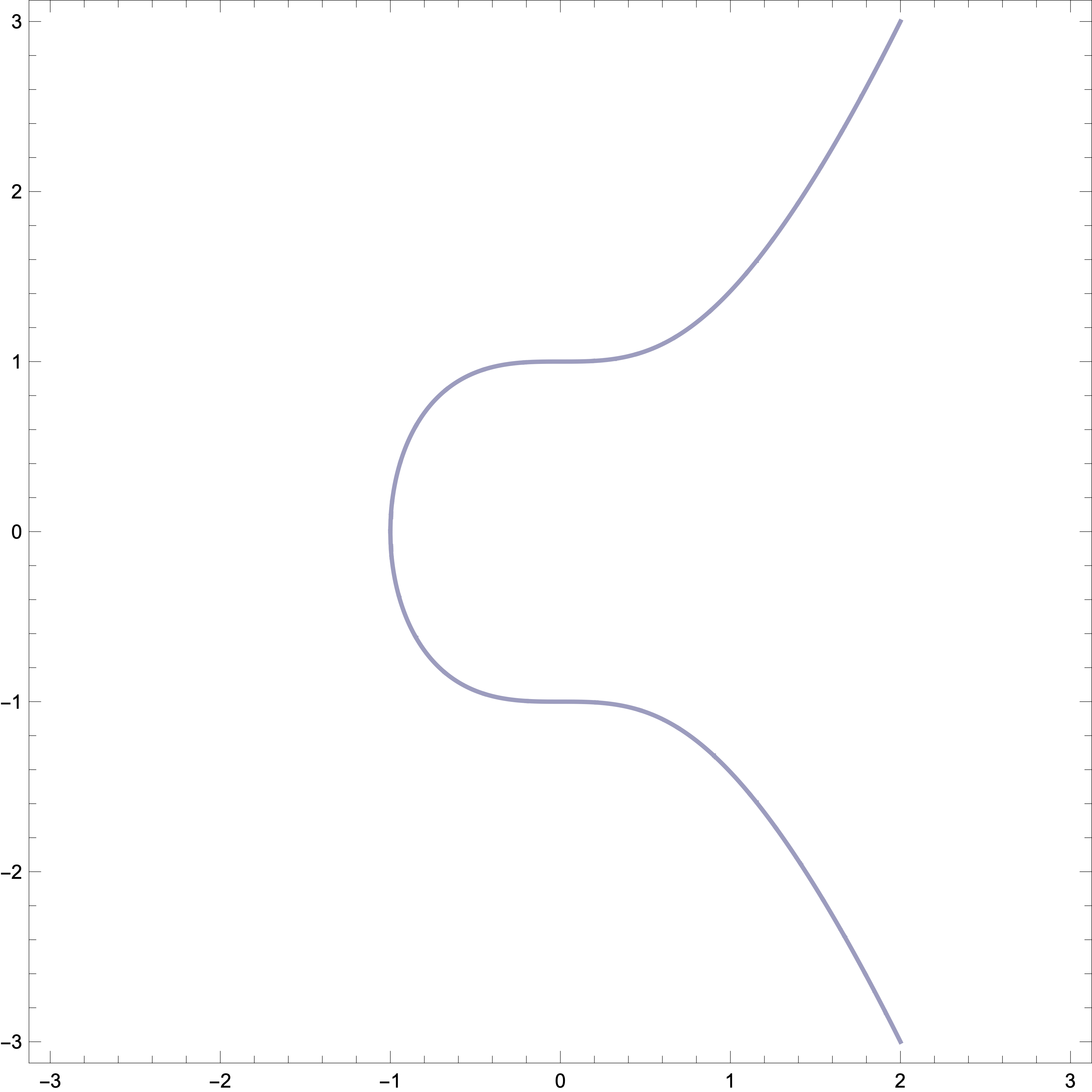
Let’s consider the elliptic curve given by the following equation:

\(y^2 = x^3 + 1\)

Over the reals, the curve looks something like this:

Next, let’s take the same curve over finite fields 𝔽_m (where m=pⁿ):

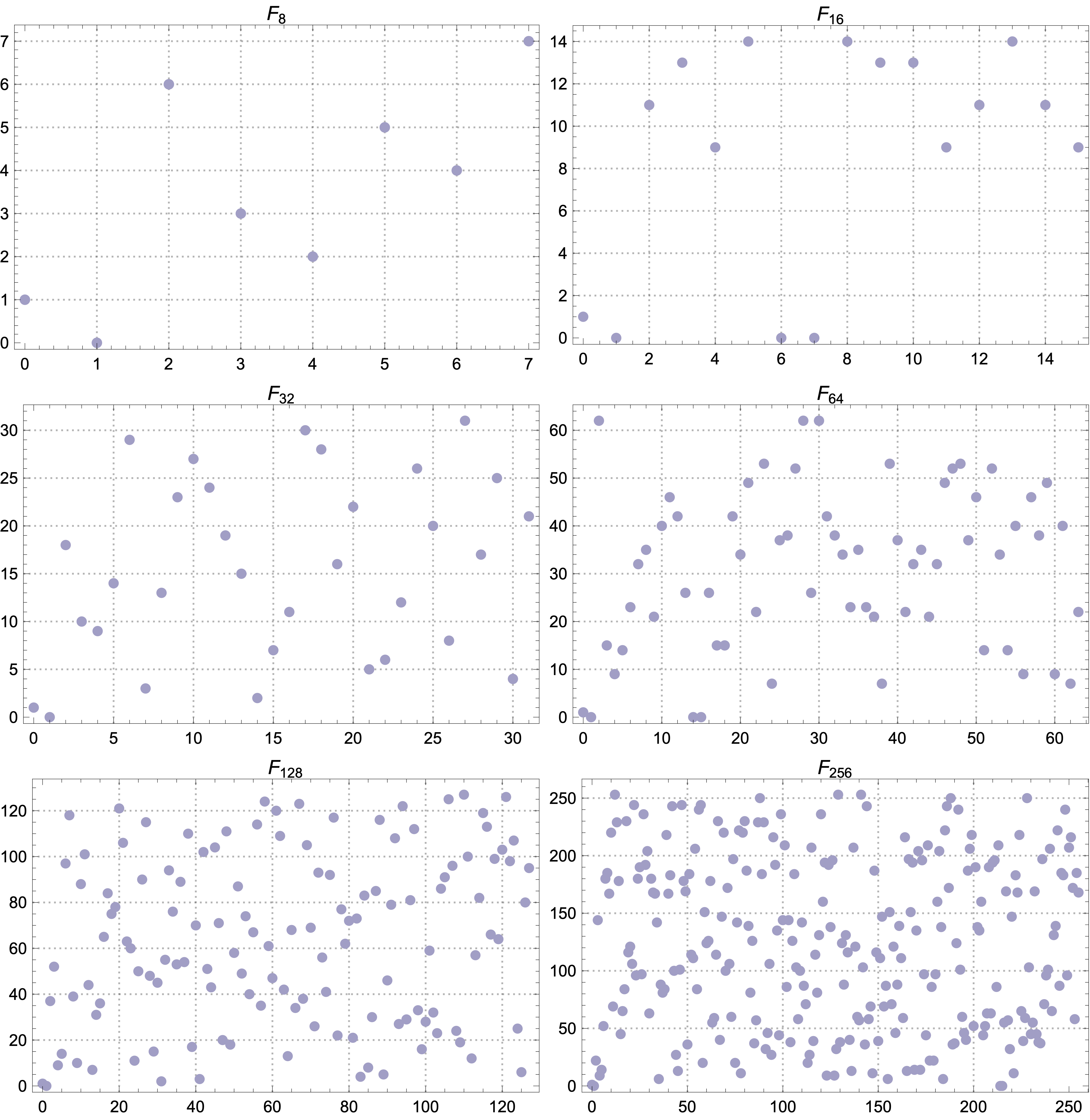
Although visually allusive, taking this particular curve over these finite fields yields predictable behavior, so far as counting solutions is concerned. This is because the number of solutions, N_m (where m = pⁿ) is dictated by the size of the field.

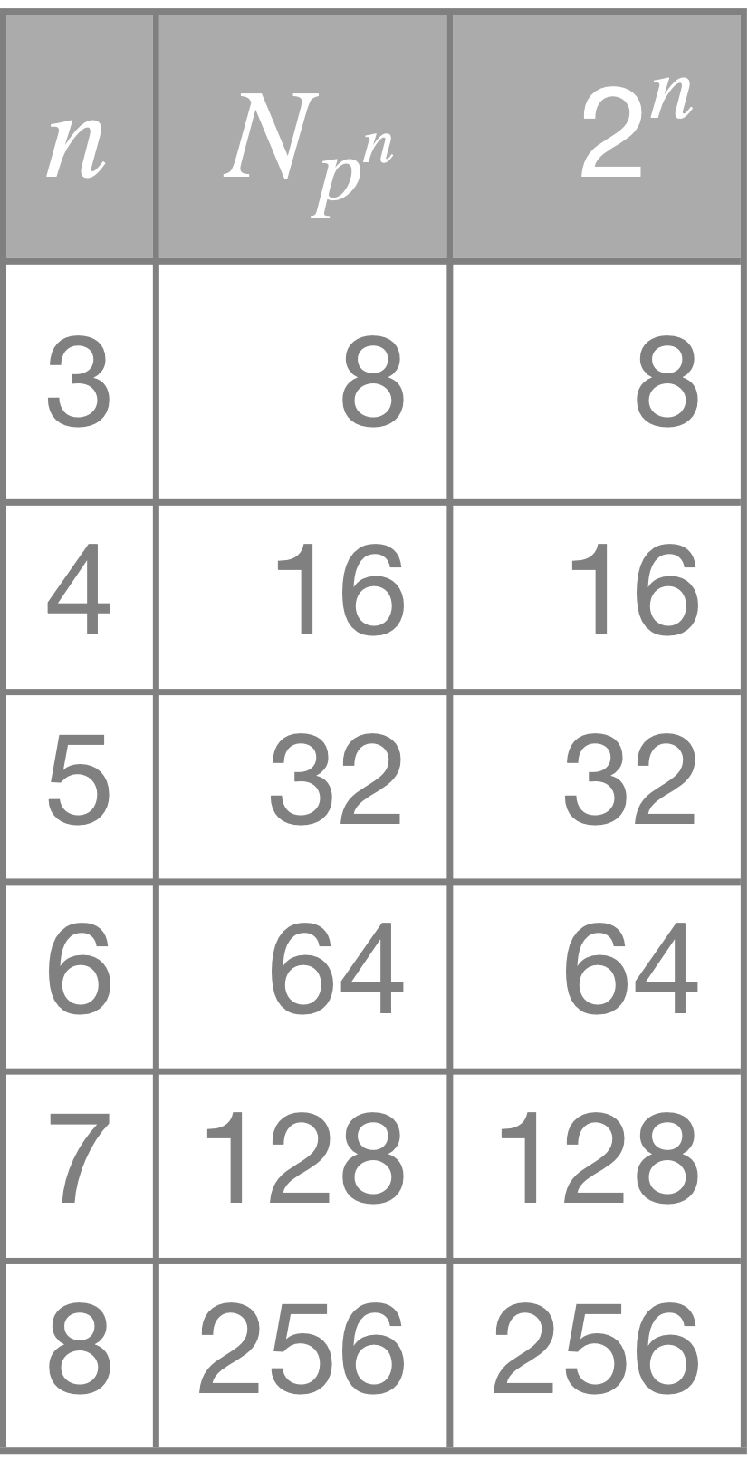
As we can see, for this curve, the number of solutions N_m is actually just the same as pⁿ! So, as a first approximation, we might suppose that N_m will be the same as pⁿ.

Motives as Geometric Corrections

However, this isn’t always the case. Consider instead the following curve:

\(y^2 = x^3 + y\)

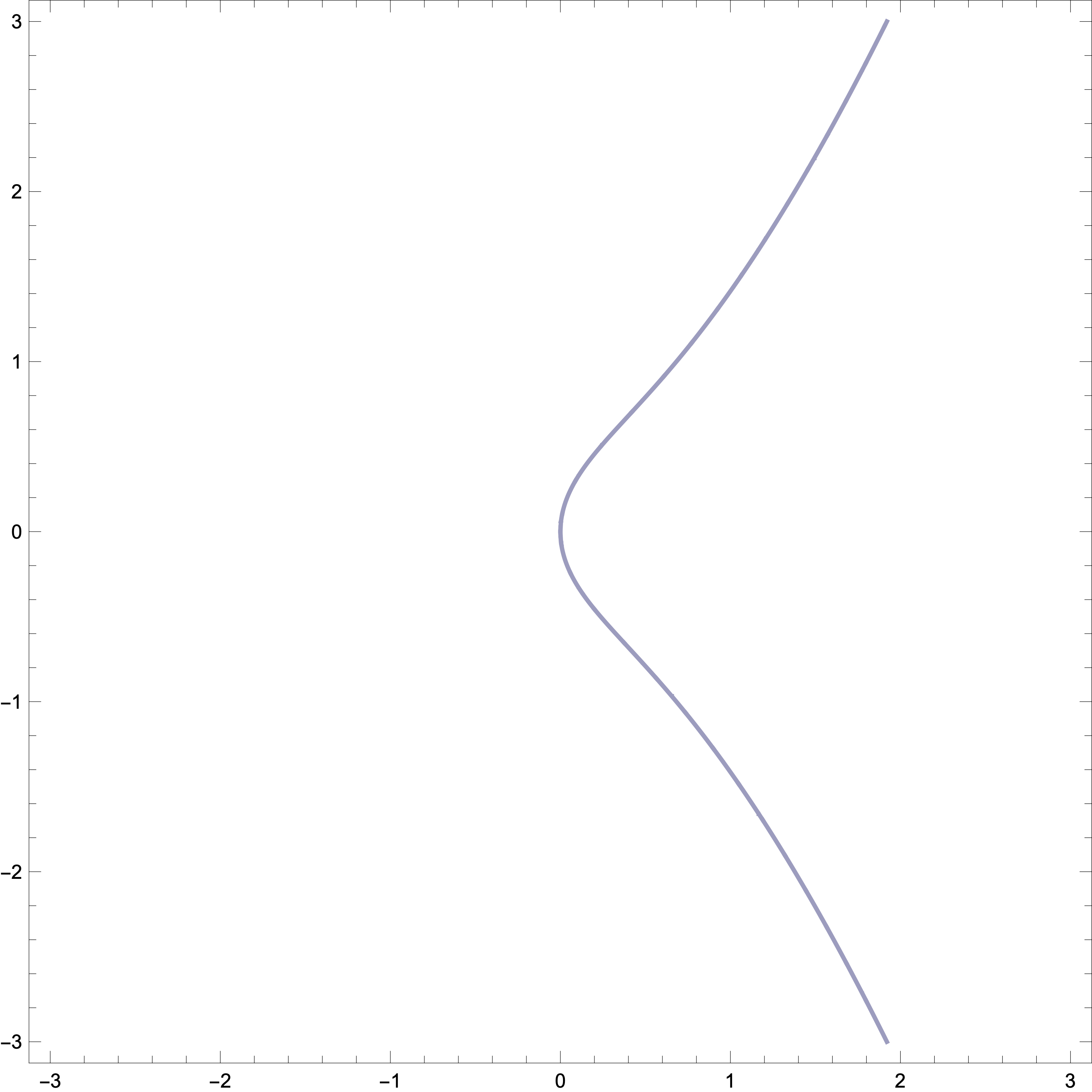
For this curve, pⁿ is just a rough approximation of N_m. Here’s a comparison of the approximation with the actual count (with the error between them highlighted). Sometimes the approximation overshoots. Sometimes it undershoots.

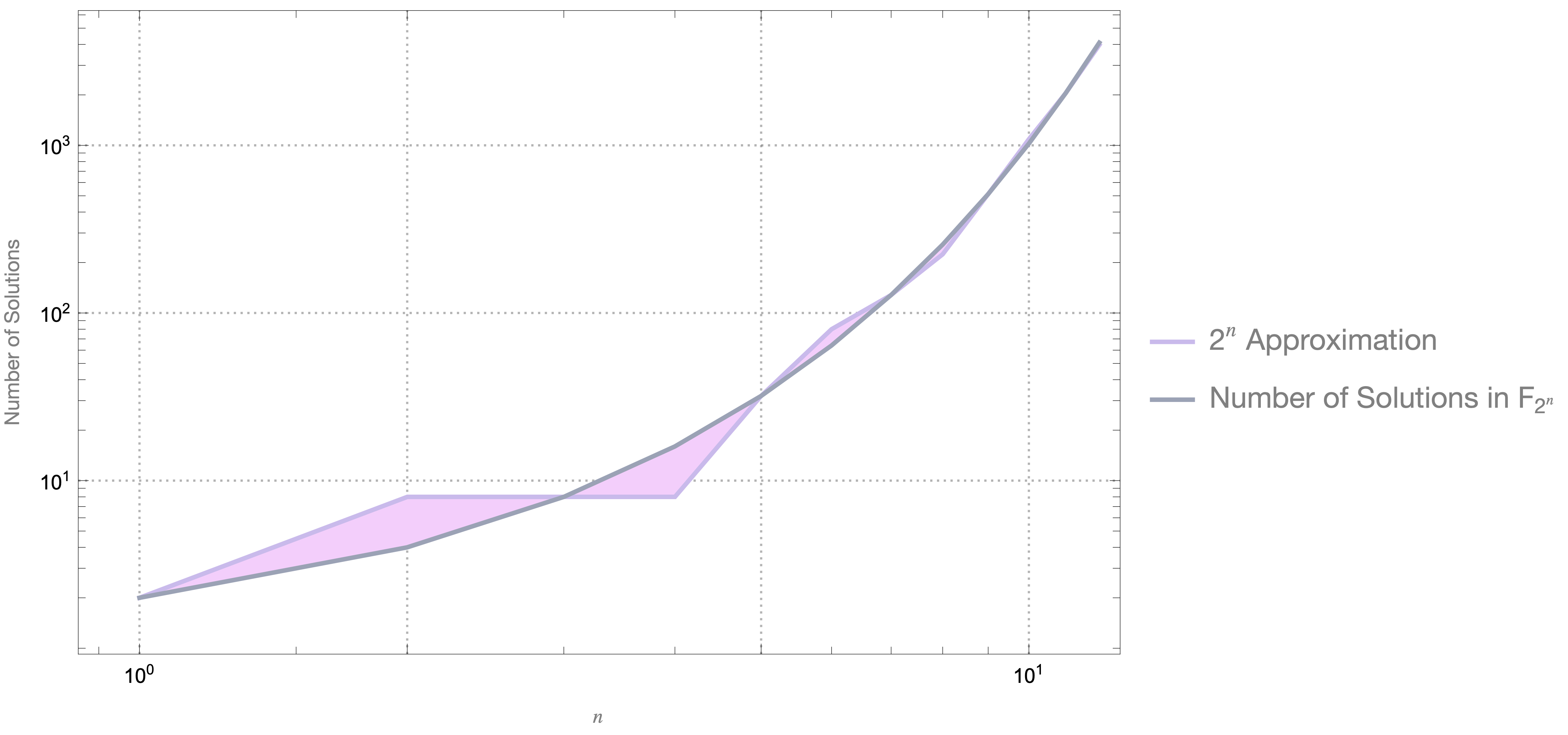
It might appear as though the errors diminish as 2ⁿ grows, but that’s just a visual artifact of the logarithmic scale. Actually, the error is growing. Here is the error term for each n:

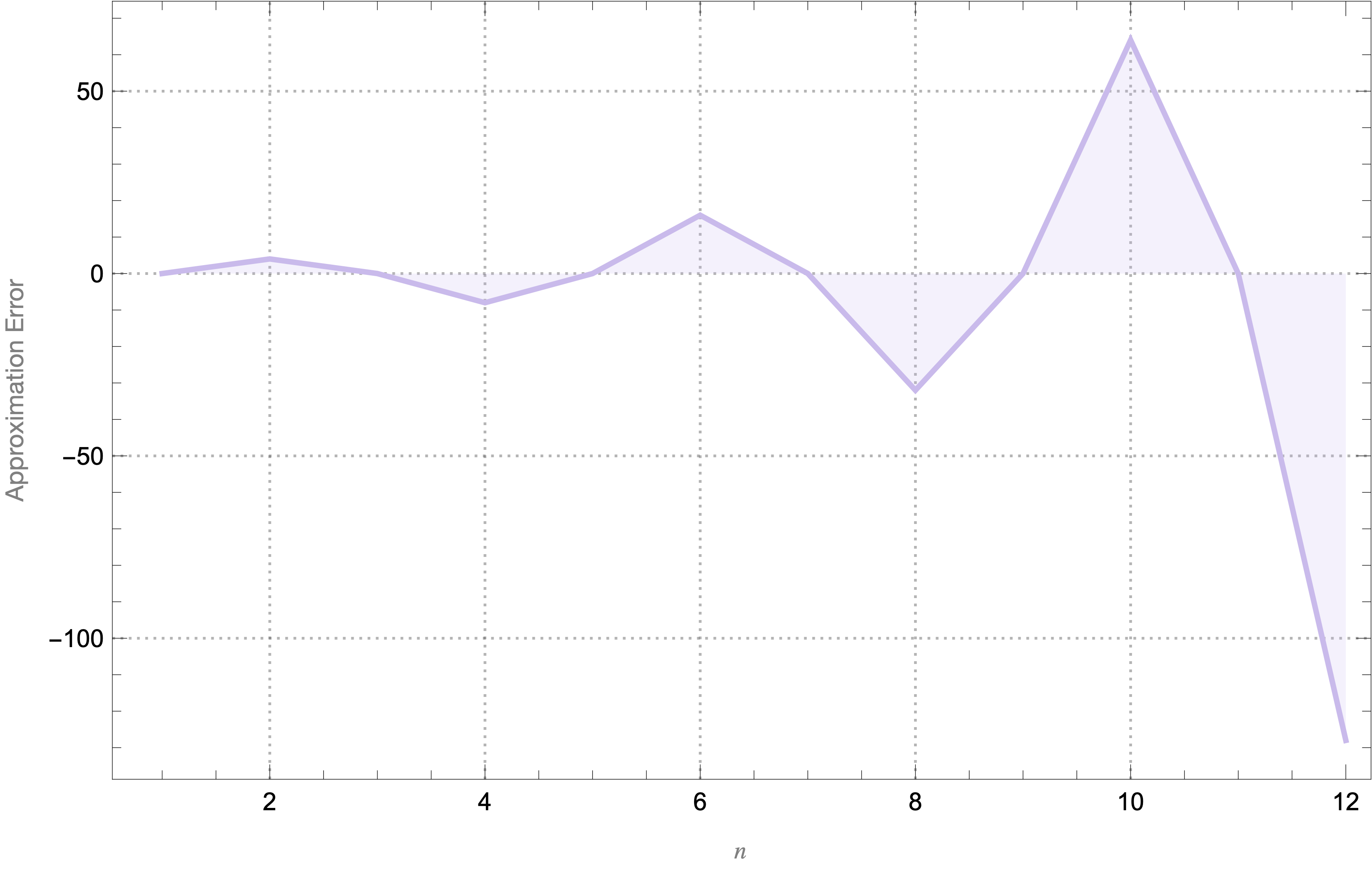
One might then ask if the ‘error term’ between the pⁿ prediction and N_m can be predicted. This is a major aspiration in modern algebraic geometry (and related research areas). In fact, it does lend itself to geometric intuition. John Baez gives a good explanation of this.

Because an elliptic curve is a torus, the pⁿ points can be interpreted geometrically as the points on some finite torus over a finite field. But what, then, is the geometric form of the error term? Alexander Grothendieck proposed a motif (or motive) as an abstract geometric object embodying this error term. It is a rather strange geometric object; for instance, in cases where the approximation ‘overshoots’ the motive will have a negative number of points.

The Hasse-Weil Zeta Function

Can one, then, construct a zeta- or L-function to introduce motivic correction terms? There is a candidate function for doing so, related to the Weil Conjectures and the Riemann Hypothesis over finite fields. First, we’ll start with the so-called “local” zeta functions. Given an algebraic variety V over a finite field 𝔽_q and its extension to 𝔽_m (where m=q^k), the local functions are given as follows:

\(Z(V,s,q) = e^{ \left( \sum_{k=1}^\infty \frac{N_k}{k} \left(q^{-s} \right)^k \right)}\)

Each function is defined for a particular q. Now, consider, for all primes, each possible local zeta function for each q=p. Taking a product of these, we can define a (global) function, the Hasse-Weil zeta-function:

\(Z(V,s,\mathbb{Q}) = \prod_p Z(V,s,p) \)

Here’s a sketch of an example of three local zeta functions (for p = 2, 3, 5) for the elliptic curve 36a1:

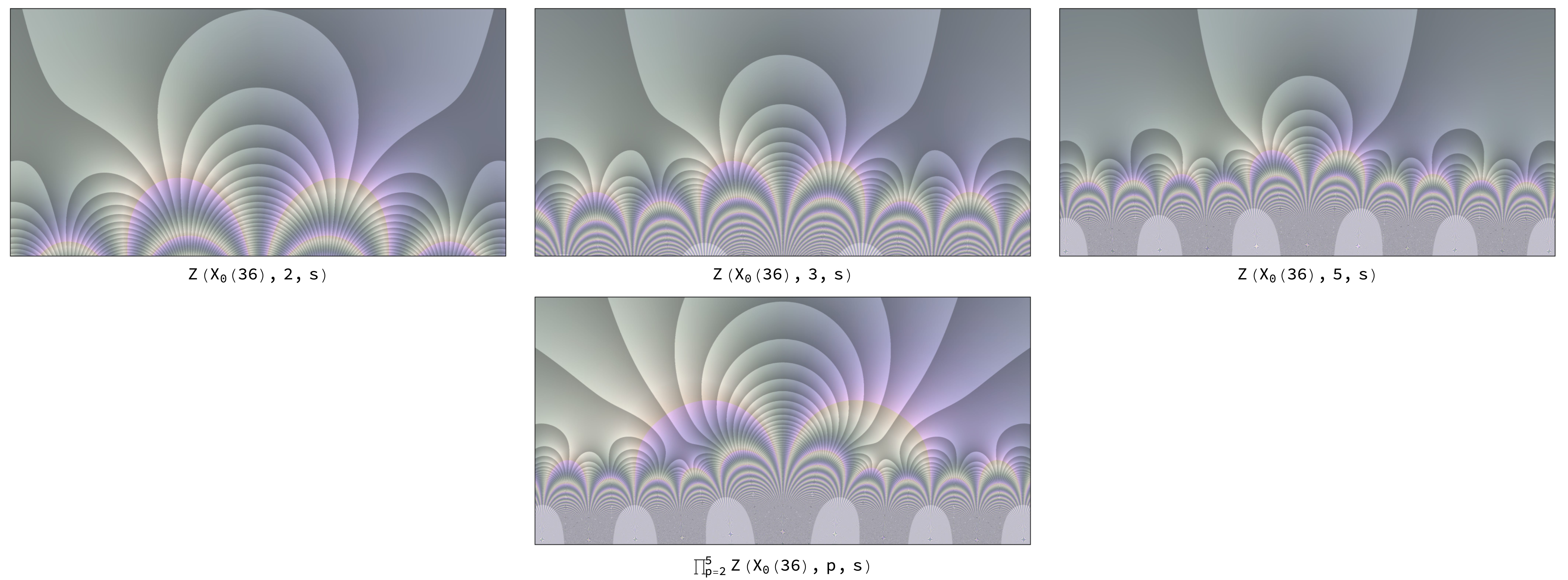
Unfortunately, analytic difficulties persist in the study of motivic L-functions. Fortunately, however, there is a modular form corresponding to elliptic curve 36a1, and it has a good L-function. A modular form is basically just an elementary example of an automorphic form, and essentially, the (arithmetic) Langlands conjectures amount to the general proposition that there exist automorphic L-functions that can be used in place of motivic L-functions (or at least, that’s one way of saying it), due to an equivalence between cusp forms and motives as arithmetic data in L-functions.

Automorphic L-Functions

Eisenstein Series and Cusp Forms

I think the best way to build intuition as to why automorphic and motivic L-functions might be equivalent, other than results such as Eichler-Shimura (discussed here) and Taniyama-Shimura, is the manner in which cusp forms, like motives, provide corrections.

The construction of automorphic L-functions with cusp forms harkens back to Robert Langlands’ early work on spectral theory and the meromorphic continuation of (the constant term of) Eisenstein series. Let’s look into what that all means.

First of all, what’s the relationship between Eisenstein series and cusp forms? In general, a space of modular forms of weight 2k can contain two components: a subspace of Eisenstein series and a subspace of cusp forms. Eisenstein series can be said to be approximations of these spaces, with cusp forms the correction terms. Langlands was working on capturing full spectra, beyond just Eisenstein series, and his work uncovered novel Euler products, i.e., new L-functions constructed from cusp forms.

Cusp Forms as Analytic Corrections

An Eisenstein series is a modular form. Whereas a general modular form f is written as

\(f \left( \frac{az + b}{cz + d} \right) = (cz+d)^k f(z) \)

an Eisenstein series of weight 2k is given as

\(G_{2k} \left( \frac{a \tau + b}{c \tau + d} \right) = (cz+d)^{2k} \sum_{(m,n) \in \mathbb{Z}^2 \setminus \{0,0\}} (m + n \tau)^{-2k} \)

In the previous section, we saw that the relationship between motives and analytic number theory is to be found in the Weil conjectures. In the case of Eisenstein series, the relationship with the Riemann zeta function is not particularly allusive. As an initial observation, one might note that ζ values appear in the definition of the q-expansion of Eisenstein series themselves:

\(E_{2k} (\tau) = 1 + \frac{2}{\zeta (1-2k)} \sum_{n=1}^\infty \frac{n^{2k-1}q^n}{1-q^n} \)

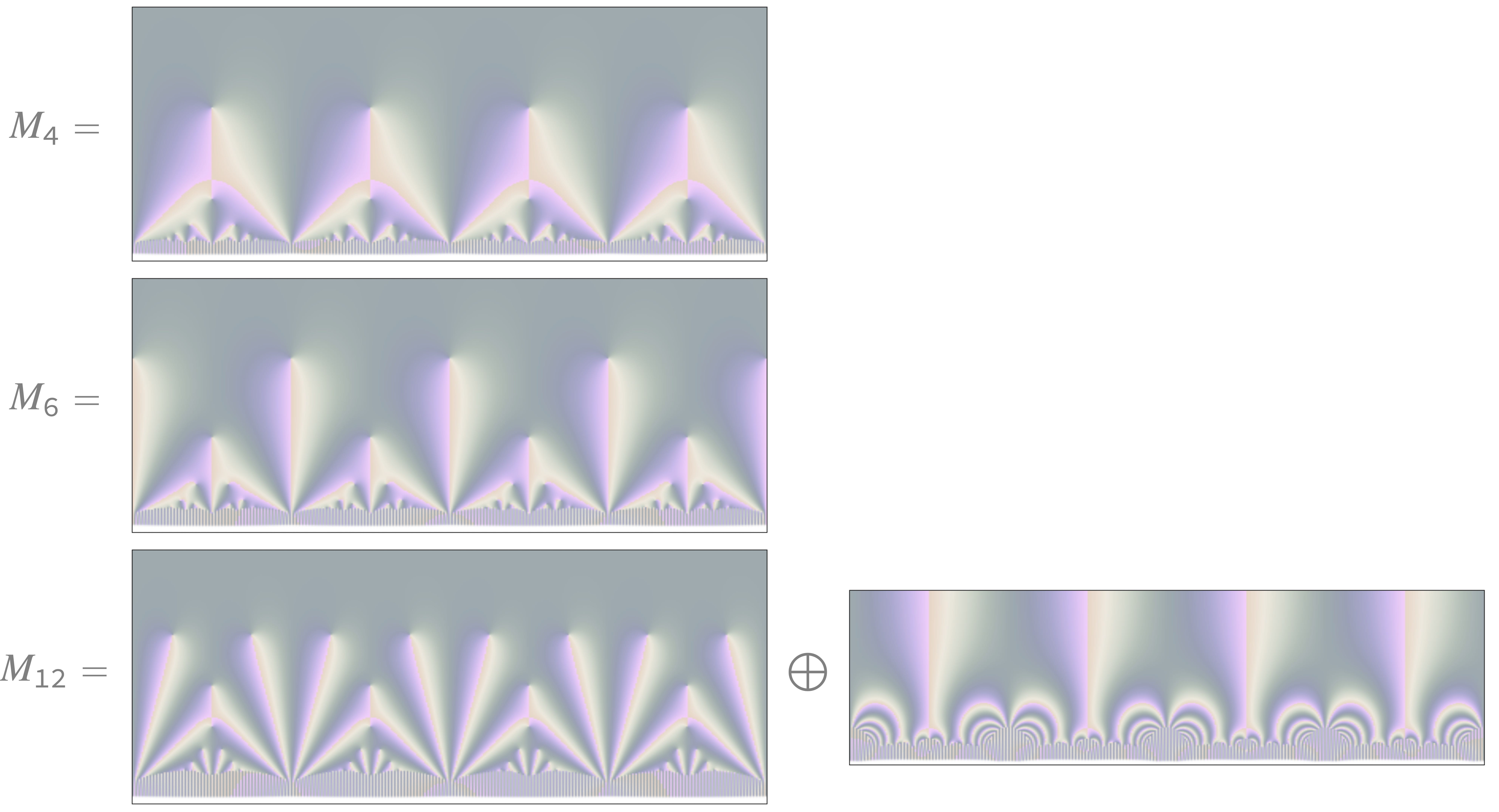
Let’s consider the space of modular forms of weight 2k in the case of SL₂(ℤ), which we’ll write as M_2k. For weights 0 ≤ 2k ≤ 10, the spaces can be described solely using Eisenstein series: M₄ using E₄; M₆ using E₆; M₈ using E₈; and M₁₀ using E₁₀. Each element of the space M_2k is just a constant multiple of the Eisenstein series E_2k. M₁₂, on the other hand, requires a cusp form. That is to say: elements of M₁₂ are not just constant multiples of E₁₂; although E₁₂ is a good approximation, a cusp form must also be added as a correction. So, unlike M₄ and M₆, M₁₂ needs a cuspidal correction:

One way of showing why the situation changes at M₁₂ is by demonstrating non-trivial arithmetic relations between modular forms of weight 12. To take a famous example, consider the difference between E₄ cubed and E₆ squared:

\(E^3_4(z) - E^2_6(z)\)

This difference has weight 12, so it is an element of M₁₂, but does not vanish; thus, they aren’t multiples of each other. Let’s look at their difference. First, here are the first few terms of their respective q-expansions:

\(E^3_4(z) =1 + 720 q + 179280 q^2 + 16954560 q^3 + 396974160 q^4 + \ldots\)

\(E^2_6(z) = 1 - 1008 q + 220752 q^2 + 16519104 q^3 + 399517776 q^4 + \ldots\)

Let’s take their difference:

\(E^3_4(z) - E^2_6(z) = 1728 q - 41472 q^2 + 435456 q^3 - 2543616 q^4 + \ldots\)

Now, suppose we were to divide this difference by 1728:

\(\frac{E^3_4(z) - E^2_6(z)}{1728} = q - 24 q^2 + 252 q^3 - 1472 q^4 + \ldots\)

Why 1728? Well, look at the coefficients of this q-expansion now. They’re the same as the coefficients of Ramanujan’s tau-function, which is a cusp form!

\(\Delta(z) = \sum_{n=1}^\infty \tau(n)q^n = q - 24 q^2 + 252 q^3 - 1472 q^4 + \ldots\)

Thus, we’ve found the error term to our E₁₂ approximation of M₁₂. It’s the cusp form:

\(E^3_4(z) - E^2_6(z) = \Delta(z)\)

Thus, we can say that E₁₂ is only an approximation of M₁₂, which is corrected with Δ(z):

\(M_{12} = \mathbb{C} \cdot E_{12} \oplus \mathbb{C} \cdot \Delta\)

Adeles and Automorphic L-Functions

Cusp forms are key data in the Euler factors of so-called automorphic L-functions. One might ask why automorphic L-functions are believed to have better analytic properties than their motivic counterparts. That’s a somewhat complicated topic, but one elementary comparison with the Hasse-Weil case can be given.

Automorphic L-functions are constructed using adeles. From an arithmetic perspective, and for those interested in Diophantine geometry, adeles are quite intriguing. In order to explain why, I should first introduce the local-global principle in arithmetic geometry, which says that

For any curve defined by a set polynomials with rational coefficients, if it has (a) solution(s) over the p-adic fields (for all p) and a solution over the reals, then it also has a solution over the rationals.

Adeles provide a useful way to exploit the local-global principle, as they offer a way to work with all completions of the rationals at once:

\(\mathbb{A}_{\mathbb{Q}} = \mathbb{R} \times \prod_p \mathbb{Q}_p\)

Recall that our Hasse-Weil functions had a somewhat similar structure, i.e., a product over all local functions. The introduction of adeles into L-functions harkens back to Tate’s thesis. Modular forms can be treated as automorphic forms on the group GL₂(𝔸), and more broadly, automorphic forms generalize to GL_n(𝔸). Fortunately, for automorphic representations, the local data uniquely determine the global data. Thus, the Euler factors in an automorphic L-function, thanks to adeles and the properties of automorphic representations, exploit the local-global principle nicely.

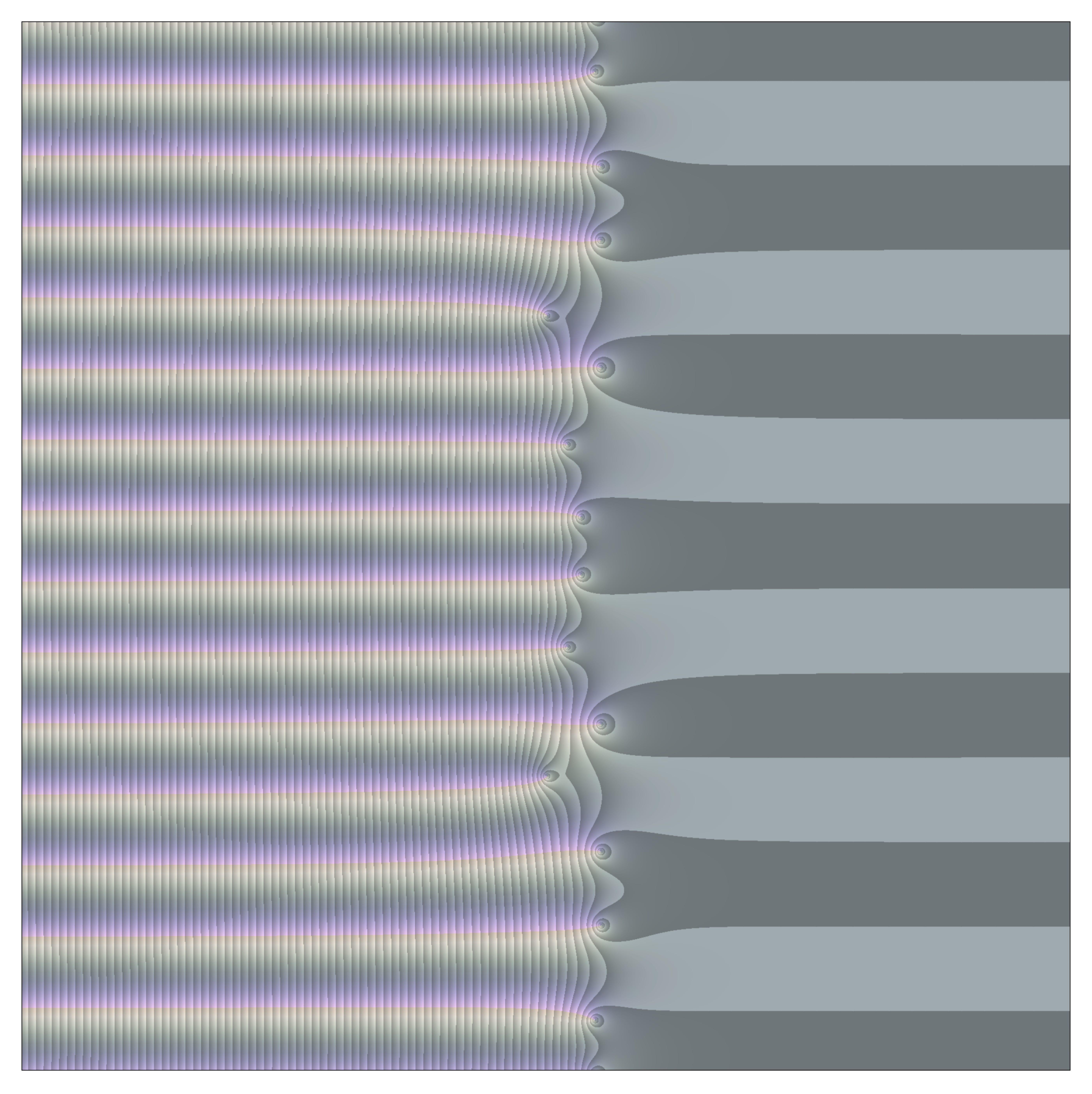
So, let’s return to our original elliptic curve, 36a1. Its corresponding modular form, 36.2.2.a, admits the following L-function:

\(1− 4 \times 7^{-s} + 2 \times 13^{-s} + 8 \times 19^{-s} − 5\times 25^{-s} − 4\times31^{-s} − 10 \times 37^{-s} + 8 \times 43^{-s} +\)

\( 9 \times 49^{-s} + 14 \times 61^{-s} − 16 \times 67^{-s} − 10 \times 73^{-s} − 4\times79^{-s} − 8\times91^{-s} + \)

\(14\times97^{-s} + 20\times103^{-s} + 2 \times 109^{-s} + \ldots\)

plotted below:

What’s nice about this is that we don’t have to compute the error term for all mod pⁿ, nor do we need to take a product of local zeta functions.